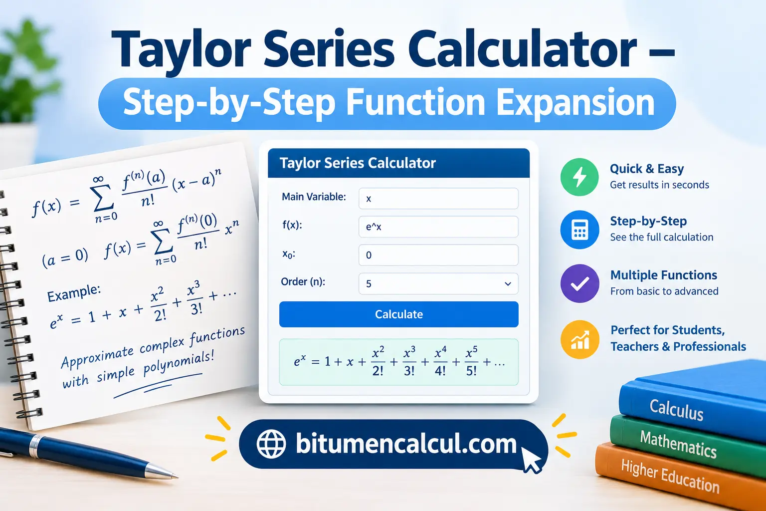
Taylor Series Calculator – Step-by-Step Function Expansion

This online Taylor Series expansion calculator makes it easier to approximate functions near a chosen point. It works by expressing a function as a series of polynomial terms, helping users understand its behavior in a specific region more clearly. This tool is particularly helpful for students, teachers, and professionals who want to explore and analyze complex functions in a simpler, more practical way.

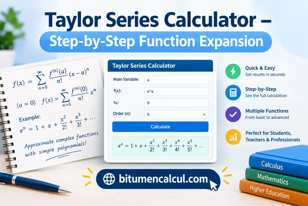
How to Use the Taylor Series Expansion Calculator

Using the Taylor Series expansion calculator is simple. Enter the required details in the fields below to calculate the expansion:

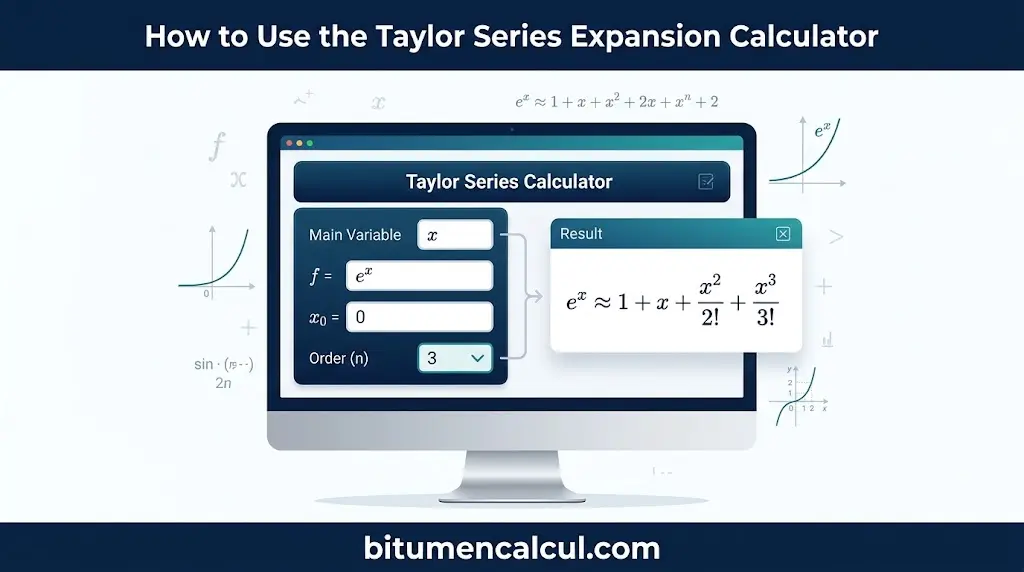
• Main Variable: Enter the variable used in your function, such as (x).
• f: Type the function you want to expand, for example, (e^x) or (\sin(x)).
• x0: Specify the point at which you want to calculate the expansion, such as (0), (1), or (\pi).
• Order (n): Choose the order of the expansion to determine how many terms are included in the approximation, such as (2) or (3).

Data Entry Guide

Follow these instructions to enter your function correctly and get an accurate result from the Taylor Series expansion calculator.

Category	Instructions and Examples
Variables	A function may contain multiple variables, but you must select only one main variable. Variables can be represented by a single uppercase or lowercase letter. For example, (f(x)=4x) has one main variable, (x). If (g(x)=4x*m+x+1) contains a secondary parameter (m), enter x in the “Main Variable” field.
Numbers	Use a dot (.) as the decimal separator when entering numbers.
Operators	Use + for addition, - for subtraction, * for multiplication, / for division, and ^ for powers. For multiplication, enter a*b rather than a.b or ab. For example, type 2*x to represent (2x).
Constants	You can use pi to represent (\pi) (approximately 3.14) and e for Euler’s number (approximately 2.72). For example, enter pi*x or e*(x+1+2*e)^2.
Common Functions	The calculator supports sqrt(x) for the square root, exp(x) for the exponential function, and log(x) or ln(x) for the natural logarithm.
Trigonometric Functions	You can use sin (sine), cos (cosine), tan (tangent), cot (cotangent), sec (secant), and csc (cosecant) in your function.
Inverse Trigonometric Functions	Supported functions include arcsin (arcsine), arccos (arccosine), arctan (arctangent), arccot (arccotangent), arcsec (arcsecant), and arccsc (arccosecant).
Hyperbolic Functions	You can use sinh (hyperbolic sine), cosh (hyperbolic cosine), tanh (hyperbolic tangent), coth (hyperbolic cotangent), sech (hyperbolic secant), and csch (hyperbolic cosecant).
Inverse Hyperbolic Functions	The calculator supports asinh (inverse hyperbolic sine), acosh (inverse hyperbolic cosine), atanh (inverse hyperbolic tangent), acoth (inverse hyperbolic cotangent), asech (inverse hyperbolic secant), and acsch (inverse hyperbolic cosecant).

Tip: Enter each function and operator using the specified format. Writing expressions correctly helps the calculator interpret your input and calculate the Taylor Series expansion as intended.

What Is a Taylor Series?

A Taylor series expresses a function as an infinite sum of polynomial terms using the function’s derivatives at a specific point (a):

[
f(x)=\sum_{n=0}^{\infty}\frac{f^{(n)}(a)}{n!}(x-a)^n
]

When the expansion point is (a=0), the series is known as a Maclaurin series:

[
f(x)=\sum_{n=0}^{\infty}\frac{f^{(n)}(0)}{n!}x^n
]

Why is this useful? Taylor series make complex functions, such as (\sin(x)), (e^x), (\ln(x)), and (\frac{1}{1+x}), easier to approximate using polynomials. Since polynomial calculations are relatively straightforward for both humans and computers, Taylor series play an important role in numerical methods, asymptotic expansions, and approximation theory.

A Taylor polynomial of degree (n) is a finite approximation that includes terms up to ((x-a)^n). It matches the function’s value and its first (n) derivatives at the expansion point, making it useful for approximating the function near (a).

Importance and Uses of Taylor Series Expansion

Taylor series expansion is an important concept in calculus and mathematical analysis because it helps approximate how a function behaves near a particular point. It is widely used to simplify calculations involving limits, derivatives, and integrals. Taylor series also make complicated mathematical expressions easier to work with in asymptotic analysis, convergence studies, and numerical approximation methods.

Key Concepts and Rules for Calculating a Taylor Series Expansion

To calculate a Taylor series expansion, you need to find the successive derivatives of a function and evaluate them at the chosen expansion point. The Taylor–Young formula provides a way to express a function as a polynomial approximation of a given order (n) around a point (a):

[
f(x)=\sum_{k=0}^{n}\frac{f^{(k)}(a)}{k!}(x-a)^k+o((x-a)^n)
]

Here, (f^{(k)}(a)) represents the (k)-th derivative of the function evaluated at (a), while (k!) denotes the factorial of (k). The order (n) determines the degree of the polynomial approximation. This formula describes the function’s behavior near the expansion point, provided the required differentiability conditions are satisfied.

Remainder Notation: Little o

The term (o((x-a)^n)), read as “little o of ((x-a)^n),” represents the remainder that remains after the Taylor polynomial of degree (n) is calculated. It indicates that this remainder becomes negligible compared with ((x-a)^n) as (x) approaches (a). In other words, the ratio of the remainder to ((x-a)^n) approaches zero.

This calculator uses little-o notation to express the remainder for the expansion order you select. You may also encounter Landau’s big-O notation, (O((x-a)^n)), which provides an upper bound on the remainder’s magnitude. Although big-O notation is commonly used in mathematics and analysis, little-o notation more precisely indicates that the remainder is of smaller order than ((x-a)^n).

When a Taylor Series Expansion Does Not Exist

Not every function has a valid Taylor series expansion at every point. If a function does not meet the necessary conditions, the calculator reports an error instead of producing an approximation.

• No power series expansion: Some functions cannot be represented by a Taylor series at a particular point. For example, (\ln(x)) does not have a Taylor expansion at (x=0).
• Insufficient differentiability: A function may not have the derivatives required for the requested expansion order. For example, (f(x)=\sqrt[3]{x}) has a vertical tangent at (x=0), preventing a standard Taylor expansion there.

When a function has a pole at a given point, such as (\frac{1}{x}) at (x=0) or (\frac{1}{x-1}) at (x=1), the calculator may provide a generalized expansion containing negative powers, known as a Laurent series, rather than a standard Taylor series.

If the calculator reports an error, try choosing a different expansion point (a) or selecting a lower expansion order.

Taylor Series Expansion of Common Functions

Taylor series expansions represent common functions as polynomial expressions, making them easier to approximate and calculate near a specific point. Below are some widely used examples of Taylor series centered at (x=0), also known as Maclaurin series.

1. Exponential Function

The Taylor series for (e^x) is:

[
e^x=1+x+\frac{x^2}{2!}+\frac{x^3}{3!}+\cdots
]

2. Sine Function

The Maclaurin series for (\sin(x)) contains alternating odd powers of (x):

[
\sin(x)=x-\frac{x^3}{3!}+\frac{x^5}{5!}-\cdots
]

3. Cosine Function

The series for (\cos(x)) contains alternating even powers:

[
\cos(x)=1-\frac{x^2}{2!}+\frac{x^4}{4!}-\frac{x^6}{6!}+\cdots
]

4. Tangent Function

The Taylor series for (\tan(x)) begins with:

[
\tan(x)=x+\frac{x^3}{3}+\frac{2x^5}{15}+\frac{17x^7}{315}+\cdots
]

5. Natural Logarithm

The expansion of (\ln(1+x)) is:

[
\ln(1+x)=x-\frac{x^2}{2}+\frac{x^3}{3}-\frac{x^4}{4}+\cdots
]

This series converges for (-1<x\leq1).

6. Square Root Function

The Taylor series for (\sqrt{1+x}) begins with:

[
\sqrt{1+x}=1+\frac{x}{2}-\frac{x^2}{8}+\cdots
]

7. General Power Function

For a real number (a), the expansion of ((1+x)^a) is:

[
\begin{aligned}
(1+x)^a={}&1+ax+\frac{a(a-1)}{2!}x^2\
&+\frac{a(a-1)(a-2)}{3!}x^3+\cdots
\end{aligned}
]

These examples show how Taylor series can approximate different types of functions using polynomial terms. The accuracy of an approximation depends on the number of terms included and the distance from the expansion point.

Examples of Taylor Series Expansion Calculations

The following examples demonstrate how to calculate Taylor series expansions for different functions using derivatives at a chosen point. Each example uses the second-order Taylor expansion around (x=0).

Example 1: Taylor Expansion of (\cos^2(x)) Around 0

Find the Taylor series expansion of (f(x)=\cos^2(x)) up to the second order.

Step 1: Calculate the function value

At (x_0=0):

[
f(0)=\cos^2(0)=1
]

Step 2: Calculate the first derivative

Differentiate the function:

[
f'(x)=-2\cos(x)\sin(x)
]

Evaluating at (x=0):

[
f'(0)=-2\cos(0)\sin(0)=0
]

Step 3: Calculate the second derivative

Differentiate again:

[
f”(x)=-2\cos^2(x)+2\sin^2(x)
]

At (x=0):

[
f”(0)=-2
]

Step 4: Apply the Taylor formula

Using the second-order Taylor formula gives:

[
\boxed{\cos^2(x)=1-x^2+o(x^2)}
]

Example 2: Taylor Expansion of (\frac{1}{1-x}) Around 0

Calculate the Taylor series expansion of (f(x)=\frac{1}{1-x}) up to the second order.

Step 1: Calculate the function value

At (x_0=0):

[
f(0)=\frac{1}{1-0}=1
]

Step 2: Calculate the first derivative

Differentiating gives:

[
f'(x)=\frac{1}{(1-x)^2}
]

Therefore:

[
f'(0)=1
]

Step 3: Calculate the second derivative

Differentiating again:

[
f”(x)=\frac{2}{(1-x)^3}
]

Evaluating at (x=0):

[
f”(0)=2
]

Step 4: Apply the Taylor formula

Substituting these values into the second-order Taylor formula gives:

[
\boxed{\frac{1}{1-x}=1+x+x^2+o(x^2)}
]

Both examples show how evaluating a function and its derivatives at the expansion point helps construct a Taylor polynomial and approximate the function near that point.

FAQs

Conclusion

A Taylor Series expansion calculator makes it easier to approximate complex functions, understand their behavior, and solve mathematical problems step by step. By entering the function, expansion point, and desired order, you can quickly obtain a polynomial approximation without calculating every derivative manually. Whether you are studying calculus or applying mathematical concepts in science and engineering, this tool can save time, simplify calculations, and strengthen your understanding of Taylor series.

Read More:

• Simplifying Radicals Calculator
• Quilt Binding Calculator
• Quartile Calculator