Exponential Growth Calculator Calculate Growth in Seconds

Use this free exponential growth and decay calculator to easily model continuous or periodic changes. Enter the initial amount, growth or decay rate, and time to calculate the final amount. The tool also provides the growth factor, doubling time, half-life, and an Exponential growth calculator graph. For users who want a clear result with steps, it can also make the calculation easier to follow, including examples related to exponential growth calculator money.

How to calculate exponential growth

Consider this example: at the beginning of 2019, a small city had a population of 10,000 people. The population was growing at a steady rate of 5% per year. How can we calculate the projected population size for the year 2030?

From the information given, we know that the initial population, x0, is 10,000. We also know that the annual growth rate is r = 5%. To see how the Exponential growth calculator exponential function works in practice, we can use the standard formula for exponential growth:$$x(t)=10,000⋅(1+0.05)^t=10,000⋅1.05^t$$

Here, t represents the number of years that have passed since 2019. For the year 2030, we use t = 11, because there are 11 years between 2019 and 2030. Substituting this value into the formula gives:$$x(11)=10,000⋅1.05^11=17,103$$

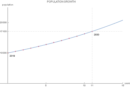
Therefore, the projected population of the city in 2030 is approximately 17,103 people.

To understand the calculation in more detail, you can use our exponential growth calculator to see the projected number of inhabitants for each year, beginning in 2019. The results are shown below, with each value rounded to the nearest whole number:

Year	t	x(t)
2019	0	10,000
2020	1	10,500
2021	2	11,025
2022	3	11,576
2023	4	12,155
2024	5	12,763
2025	6	13,401
2026	7	14,071
2027	8	14,775
2028	9	15,513
2029	10	16,289
2030	11	17,103

Looking at the population figures this way also makes the growth pattern easier to understand. You can represent the same data on a graph, using the horizontal axis for time and the vertical axis for the population value x(t). Each value from the table falls on the continuous graph of the exponential growth function:$$x(t)=10,000×1.05^t$$

Because the base of this exponential function is 1.05, which is greater than 1, the resulting exponential growth graph moves upward over time. One noticeable difference from the standard exponential function graph is that its y-intercept is not 1. Instead, it is 10,000, matching the initial population value x0.

This example also shows some possible limitations of the exponential growth model. In real-world situations, it is usually unrealistic to assume that a growth rate will stay exactly the same for a long period. For example, expecting a city’s population to increase by precisely 5% every year for more than a decade may not reflect actual population trends.

In practice, growth rates can naturally rise and fall due to many different factors, and these changes are not accounted for in a simple exponential model. A more realistic approach for population growth is the logistic growth model, which includes a carrying capacity. This represents the population’s natural growth limit and provides a better way to describe situations where growth eventually slows down.

If only two data values are known, an Exponential growth calculator given two points can also be useful for estimating the growth pattern between them. On the other hand, when growth happens continuously rather than at regular yearly intervals, a Continuous exponential growth calculator can be used with a continuous growth formula.

How to find the moment when the initial quantity reaches a given value

Returning to our small-city example, another useful question is: when can we expect the population to reach some important value? This can help with urban planning and preparing the city for future growth. For example, the city council may want to know in which year the population will become three times larger than the original 10,000 inhabitants.

In this situation, we already know the target value of x(t), but the exact value of t is unknown. We can find it by working through the Exponential population growth formula step by step:

1. Replace x(t) with 30,000 in the growth equation: 30,000 = 10,000⋅1.05^t.
2. Divide both sides of the equation by 10,000 to simplify it: 1.05^t = 3.
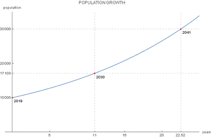
3. Take the logarithm with base 1.05 on both sides: t = log₁.₀₅3.
4. Calculate the logarithm to find the value of t: t = 22.52.

This means the population will reach approximately 30,000 people about 22.52 years after 2019. Since we are looking for the corresponding calendar year, this places the population reaching three times its original size at around 2041.

Can time be negative?

You may have noticed that exponential growth and decay models often use positive time values because they are commonly used to predict what will happen in the future. However, the formula can also work with negative time values. In that case, we are describing what happened before the initial observation was made.

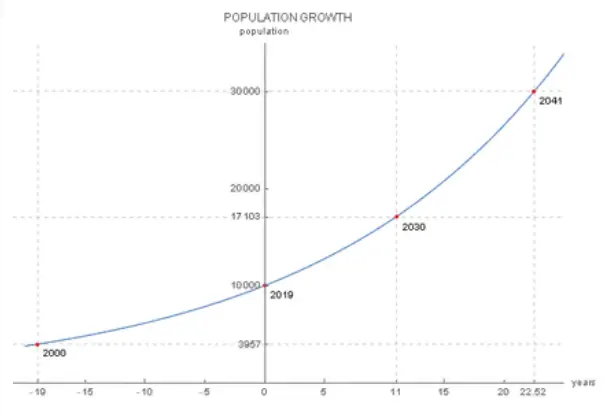
For our population example, we can use the model to ask a different question: what was the population of the small city in the year 2000 if we assume that the population growth rate was a constant 5%?

To calculate this, we use t = −19, because the year 2000 was 19 years before the initial year, 2019. Substituting this value into the formula gives:$$x(−19)=10,000⋅1.05^−19=3957$$

So, based on this exponential growth model, the city’s population in 2000 was approximately 3,957 inhabitants, as the graph below also illustrates.

An alternative way of writing the exponential growth equation

In some situations, such as when working with the exponential decay of a radioactive substance, it can be more convenient and effective to express the exponential growth and decay formula in a different form:$$x(t)=x0⋅e^{kt}$$

In this version of the equation, the coefficient k serves as the growth or decay rate, much like r does in the standard exponential growth formula. By comparing this equation with the original form, we can establish the relationship between r and k as follows:$$1+r/100=e^k$$

From this relationship, we can derive both variables. The corresponding formulas are:$$r=100⋅(e^k−1)$$

and$$k=ln(1+r/100)$$

These expressions allow you to convert between the percentage growth rate r and the exponential rate coefficient k, depending on which form of the equation is more suitable for the calculation.

Example on how to use the formula for exponential decay

Radioactive decay is one of the most common situations where the exponential decay formula is applied. When we know the initial quantity of a radioactive substance, we can use the decay law to determine how much remains after a certain amount of time. A simpler everyday example, however, is to calculate how much coffee remains in your body at 10 pm after drinking a cup of coffee at noon.

Suppose the coffee contains x0 = 95 mg of caffeine. We can use the fact that the half-life of caffeine in the human body is approximately six hours. The half-life is the amount of time required for a quantity to decrease to half of its original value. Therefore, in our example:

x(6)=1/2⋅95 mg=47.5 mg

For this calculation, the alternative form of the exponential growth and decay equation is more convenient:

x(t)=95⋅e^{kt}

Let’s work through the calculation step by step:

1. Substitute x(6)=47.5 and t=6 into the equation: 47.5=95⋅e^{6k}.
2. Divide both sides by 95 and then apply the natural logarithm. This gives: 6⋅k=ln⁡0.5.
3. Solving for k gives: k=−0.1155.
4. We can now write the exponential decay equation for this example as: x(t)=95⋅e^{−0.1155⋅t}.
5. Since 10 pm is 10 hours after noon, we need to evaluate the formula at t=10. Therefore: x(10)=95⋅e^{−0.1155⋅10}=29.9305.

So, at 10 pm, approximately 30 mg of caffeine would remain in the body according to this exponential decay model.

What if there’s no time at all?

Time can be measured using almost any suitable unit, depending on the problem. In some cases, seconds may be appropriate, while other situations may require years. You should choose the time unit according to the nature of the process you are studying. For instance, when analyzing how a city’s population changes, years would usually be the most useful unit. In contrast, when calculating how much caffeine remains in your body after drinking coffee, hours or even minutes may be more practical.

It is also important to remember that t does not necessarily have to represent time. In some applications, the variable used to measure the rate of change may be something other than time. For example, when examining how atmospheric pressure changes as altitude increases, the changing variable is distance rather than time. In that case, meters would be the appropriate unit for measuring the change.

How different exponential growth rates affect growth

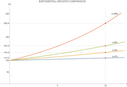
The exponential growth rate r can have a significant impact on how quickly a quantity increases from its starting value. To see this effect more clearly, let’s begin with x0 = 100 and use the exponential growth calculator to find the value of x(10) for four different growth rates:

r	x0	x(10)
1%	100	110.5
3%	100	134.4
5%	100	162.9
10%	100	259.4

As the table shows, every example starts with the same initial value, x0 = 100, yet the resulting values of x(10) are quite different. Your intuition may be misleading here, because the difference between a 1% and 3% growth rate seems relatively small at first. However, after ten periods, the value of x(10) for 3% growth is already 21.67% higher than the value produced by 1% growth.

The difference becomes even more noticeable when comparing 10% growth with 5% growth. In that case, the value is 59.23% higher for the 10% growth rate. This shows how even a seemingly small change in the exponential growth rate can produce a much larger difference over time.

You can see this effect more clearly in the following graphical representation of the four exponential growth functions:

What are real-world applications of the exponential growth?

The exponential growth and decay formula is used to describe and model many different real-world processes. Some common examples include:

• Growth of bacteria, viruses, plants, animals, and human populations;
• Decay of radioactive substances;
• Changes in the concentration of drugs in the bloodstream;
• Atmospheric pressure at different altitudes;
• Compound interest and economic growth;
• Radiocarbon dating; and
• The increasing processing power of computers and other technologies.

💡 And did you know that…

You can check whether a given set of numbers follows an exponential growth pattern by using the well-known Benford’s law.

FAQs

Conclusion

Exponential growth and decay help you understand how a quantity changes over time, whether you are tracking population, money, caffeine, or other real-world processes. With an exponential growth calculator, you can quickly calculate future values, compare growth rates, and understand these changes through formulas and graphs.

Read More:

• Mean Median Mode Calculator
• Divorce Buyout Calculator
• Speed Calculator